tutorial_lfq
Label-free quantification with FragPipe
This tutorial demonstrates label-free quantification with match-between-runs using a dataset published in Proteomics separates adult-type diffuse high-grade gliomas in metabolic subgroups independent of 1p/19q codeletion and across IDH mutational status (ProteomeXchange identifier PXD024427). In this study, researchers studied high-grade adult-type diffuse gliomas are malignant neuroepithelial tumors with poor survival rates in combined chemoradiotherapy. They used MS1-based label-free quantification (LFQ) mass spectrometry to characterize 42 formalin-fixed, paraffin-embedded (FFPE) samples from IDH-wild-type (IDHwt) gliomas, IDH-mutant (IDHmut) gliomas, and non-neoplastic controls.
In this tutorial, we will use just 6 samples, 3 IDHmut and 3 IDHwt. We will use mzML files, although Raw files can be used instead. The files can be downloaded from here
Tutorial contents
- Open FragPipe
- Load the data
- Load the LFQ-MBR workflow
- Fetch a sequence database
- Inspect the search and quantification settings
- Set the output location and run
- Inspect the results
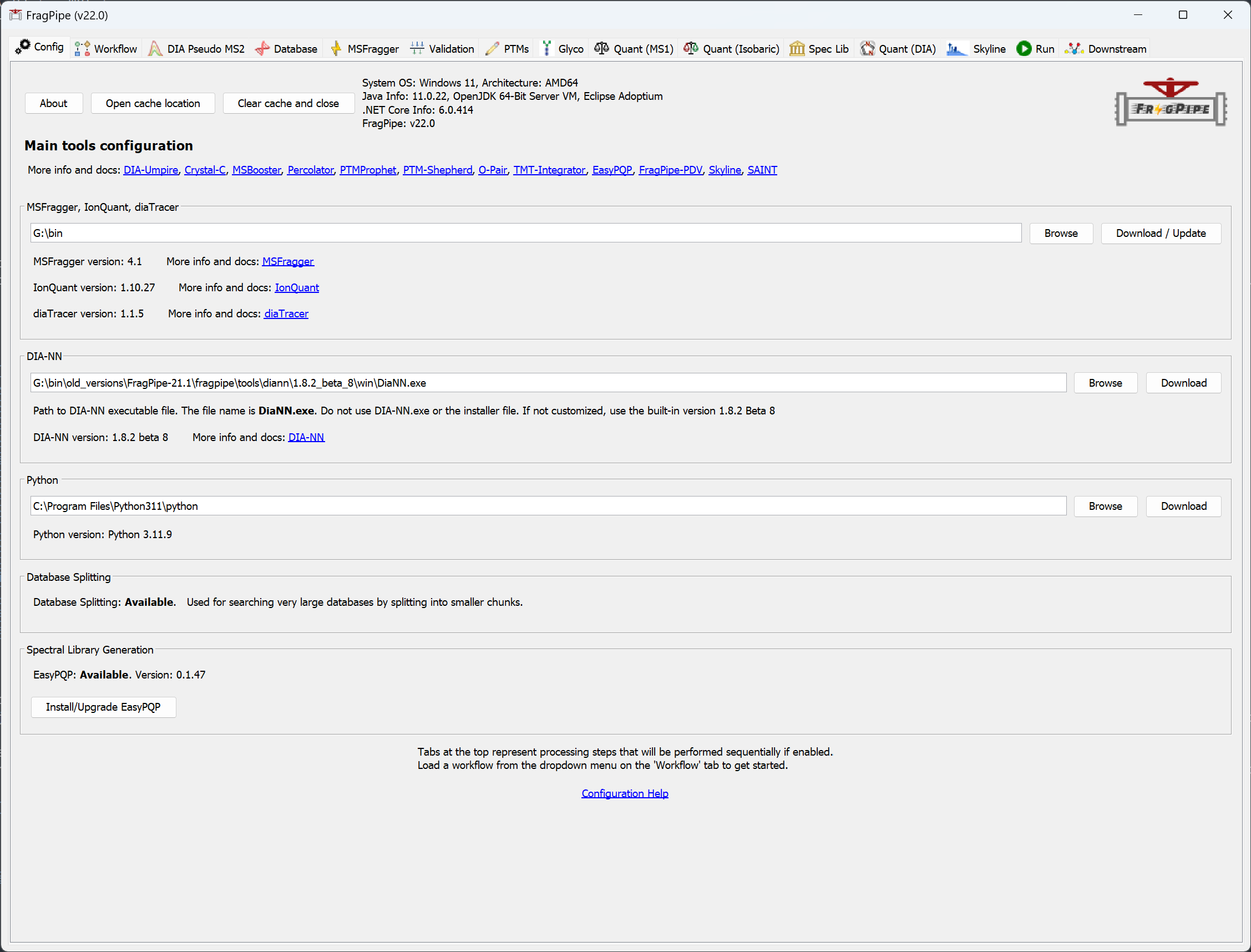
Open FragPipe
When you launch FragPipe, check that MSFragger, IonQuant, and Philosopher are configured. (If you haven’t downloaded them yet, use their respective ‘Download / Update’ buttons. Please see the tutorials here and here. Python is not needed for these exercises.)
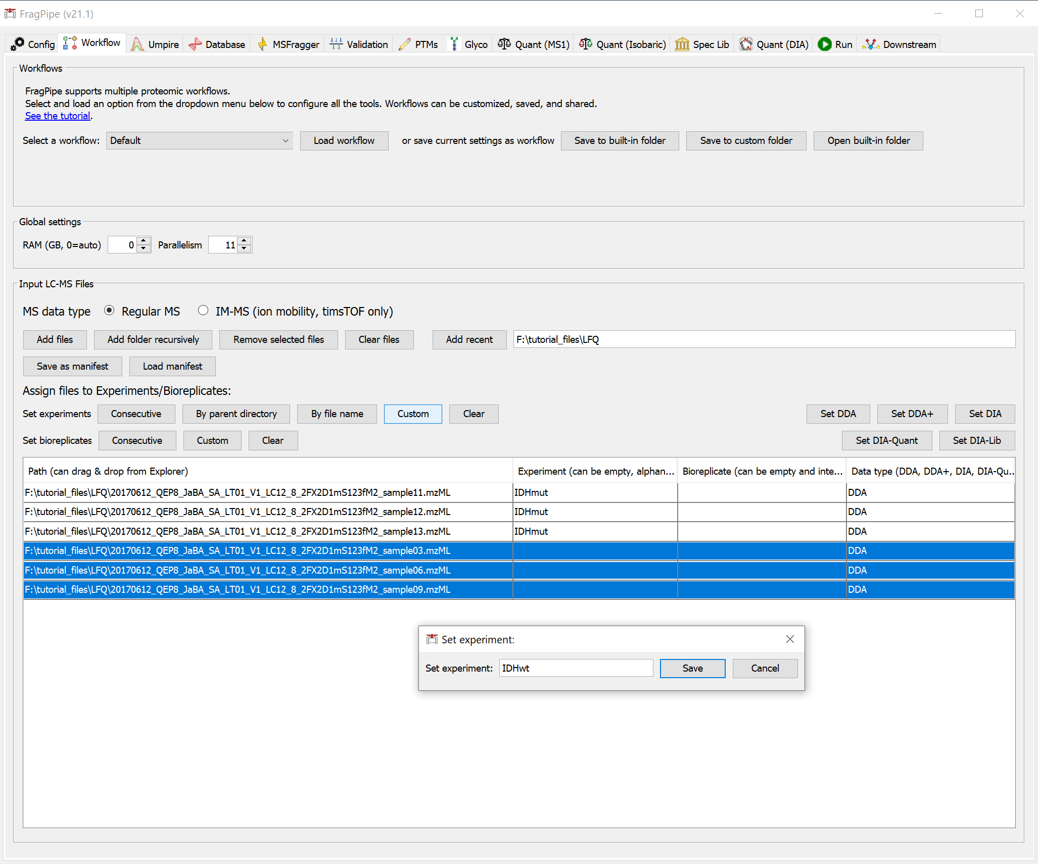
Load the data
On the ‘Workflow’ tab, drag and drop the six .raw spectral files or use the ‘Add files’ button to browse for them. We are using a subset of the full dataset with annotations shown below.
| Path | experiment | bioreplicate | data type |
|---|---|---|---|
| 20170612_QEP8_JaBA_SA_LT01_V1_LC12_8_2FX2D1mS123fM2_sample11.mzML | IDHmut | 1 | DDA |
| 20170612_QEP8_JaBA_SA_LT01_V1_LC12_8_2FX2D1mS123fM2_sample12.mzML | IDHmut | 2 | DDA |
| 20170612_QEP8_JaBA_SA_LT01_V1_LC12_8_2FX2D1mS123fM2_sample13.mzML | IDHmut | 3 | DDA |
| 20170612_QEP8_JaBA_SA_LT01_V1_LC12_8_2FX2D1mS123fM2_sample03.mzML | IDHwt | 4 | DDA |
| 20170612_QEP8_JaBA_SA_LT01_V1_LC12_8_2FX2D1mS123fM2_sample06.mzML | IDHwt | 5 | DDA |
| 20170612_QEP8_JaBA_SA_LT01_V1_LC12_8_2FX2D1mS123fM2_sample09.mzML | IDHwt | 6 | DDA |
Once you’ve added the files, you can annotate them by editing the ‘Experiment’ and ‘Bioreplicate’ fields manually or in batches with the ‘Custom’ button. The data type should be automatically detected as DDA.
Load the LFQ-MBR workflow
Still on the ‘Workflow’ tab, select the LFQ-MBR workflow from the dropdown menu, then click ‘Load’.
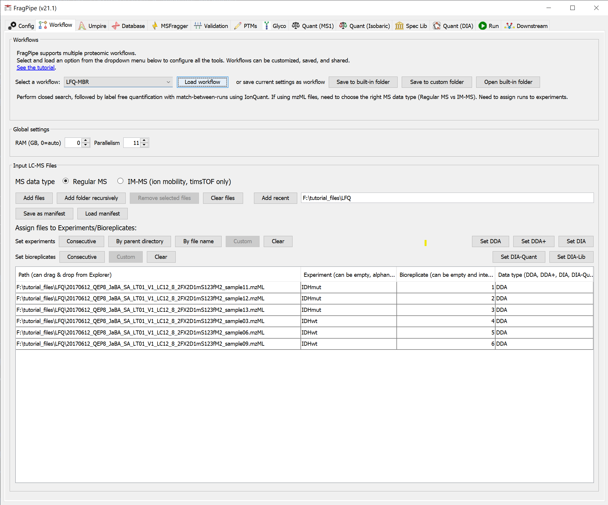
This sets all the analysis steps for a closed database search with MSFragger, rescoring with MSBooster and Percolator, protein grouping with ProteinProspector, and filtering with Philosopher, and label-free quantification with FDR-controlled match-between-runs with IonQuant.
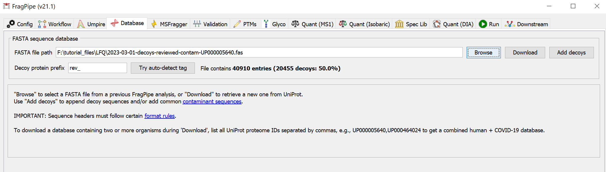
Fetch a sequence database
On the ‘Database’ tab, click ‘Download’, which will prompt you to first set the download options. We will keep the default options (human, reviewed sequences, add common contaminants) for this dataset.
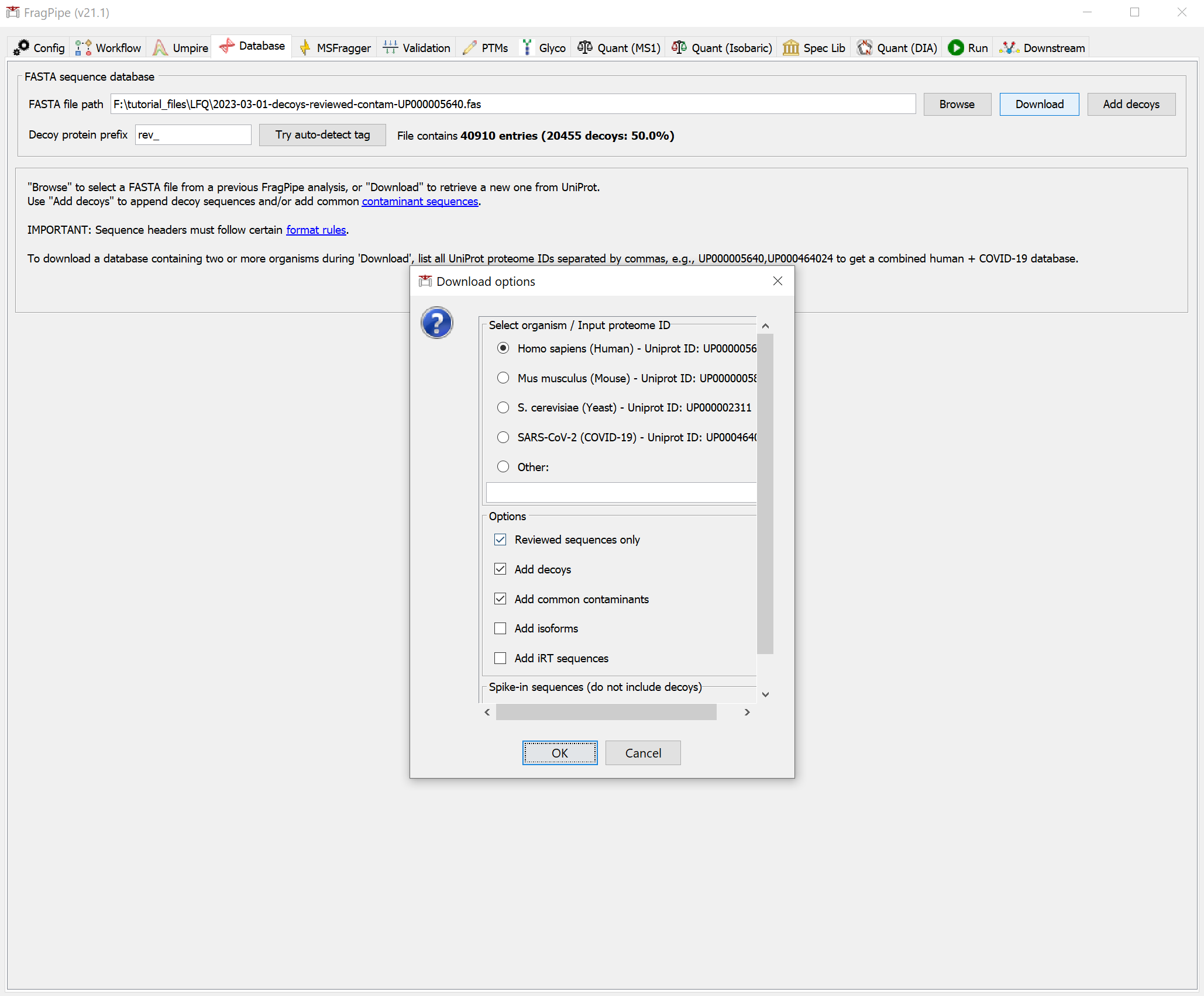
Clicking 'OK', and then, it will show the dialog for choosing a file location to store the database. Once you’ve chosen a folder, click ‘Select directory’ to start the downloading. When it’s finished, you should see that the FASTA file path now points to the new database.
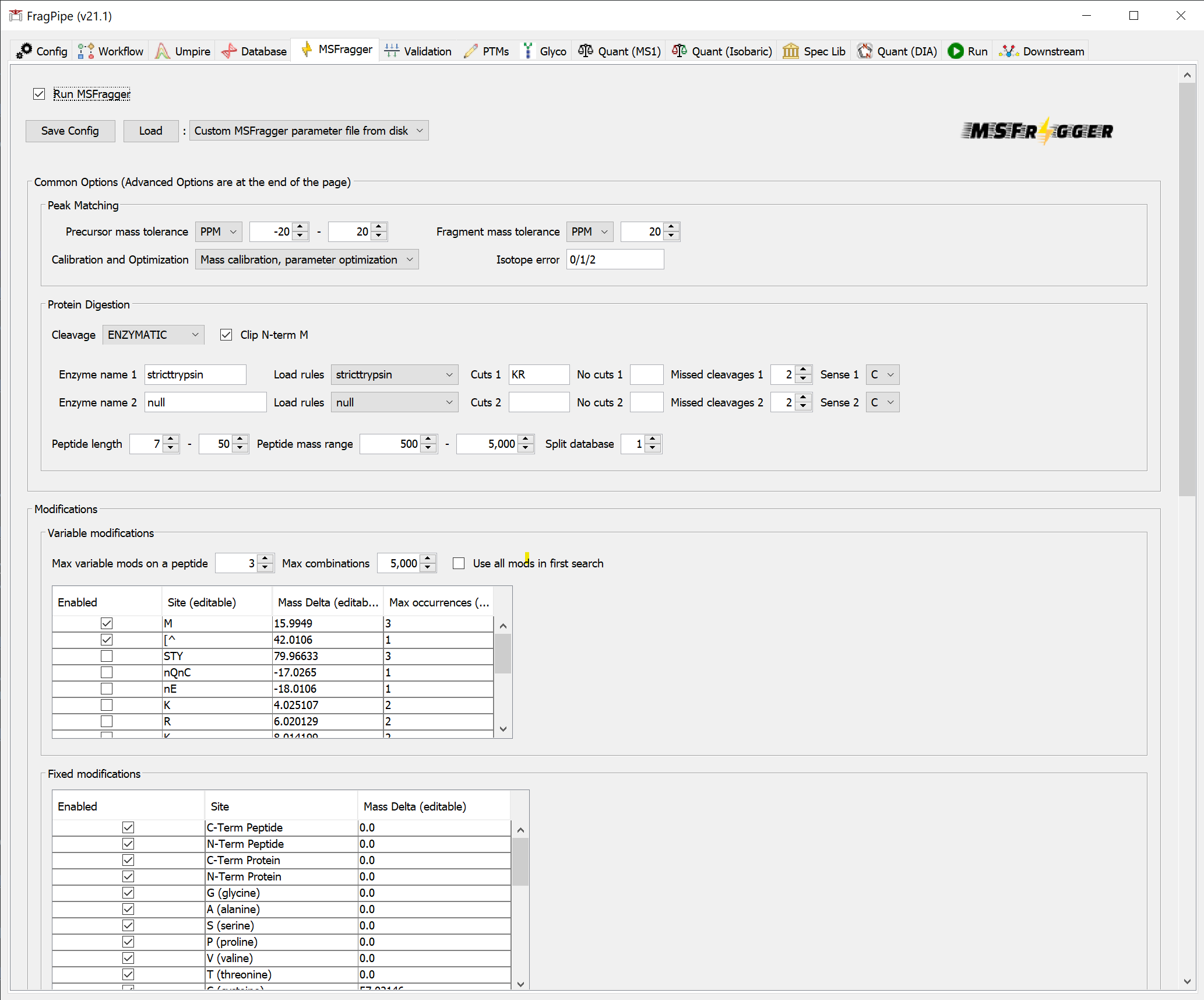
Inspect the search and quantification settings
On the ‘MSFragger’ tab, you can see the parameters that have been set by loading the workflow.
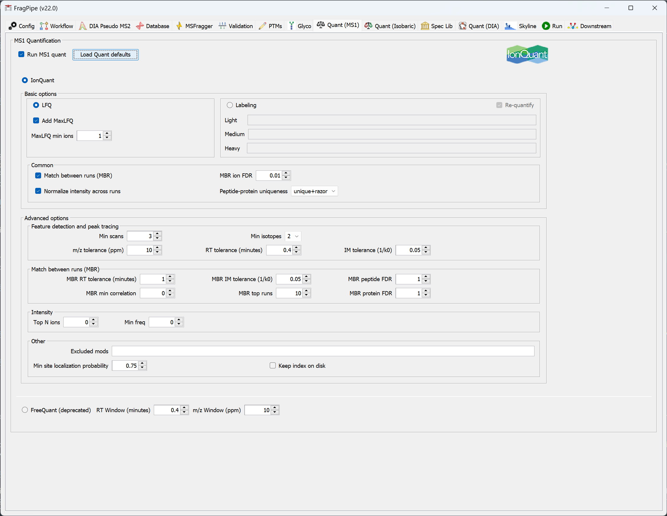
On the ‘Quant (MS1)’ tab, you can see the settings that will be used for label-free quantification. Note that IonQuant will be used and ‘Match between runs (MBR)’ is enabled. The 'MaxLFQ' quantification method is selected by default, and MaxLFQ values will be reported in addition to abundances calculated using the topN method.
Set the output location and run
On the ‘Run’ tab, use ‘Browse’ to make a new folder for the output files. Then click the ‘RUN’ button to start the analysis.
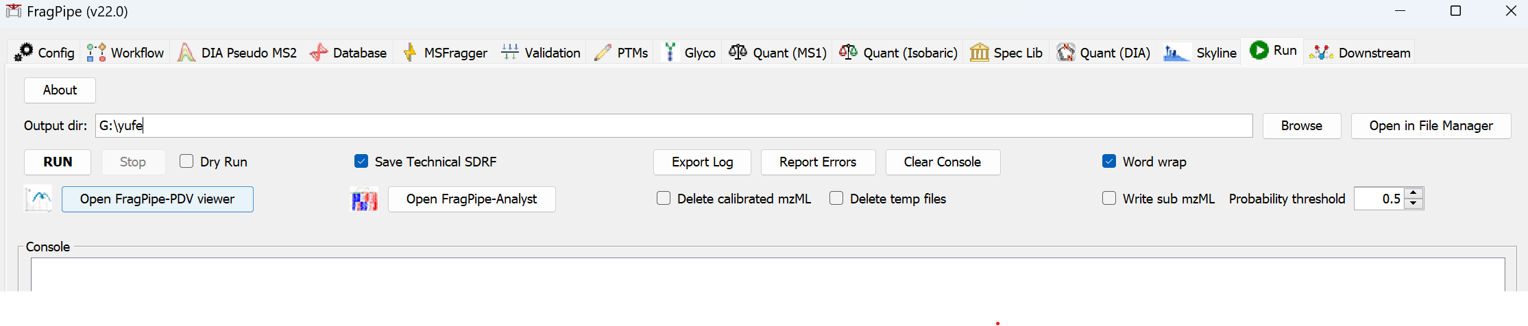
When the run is finished, ‘DONE’ will be printed at the end of the text in the console.
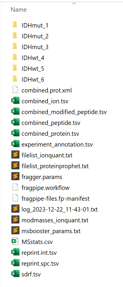
Inspect the results
In the output location, you will find combined reports (including the ‘MSstats.csv’ table, compatible with MSstats) as well as folders for each sample.
A guide to output files, with descriptions of each column in the reports, can be found here.
A more comprenehsived tutorial from the US HUPO 2023 short course
The tutorial file can be found from here
Key References
Yu, F., Haynes, S. E., Teo, G. C., Avtonomov, D. M., Polasky, D. A., & Nesvizhskii, A. I. (2020). Fast quantitative analysis of timsTOF PASEF data with MSFragger and IonQuant. Molecular & Cellular Proteomics, 10(9), 1575-1585.
Yu, F., Haynes, S. E., & Nesvizhskii, A. I. (2021). IonQuant enables accurate and sensitive label-free quantification with FDR-controlled match-between-runs. Molecular & Cellular Proteomics, 20, 100077.